Computing the Signal-to-Noise Ratio (SNR) for SCA
This tutorial and accompanying notebook aim to give the reader the tools to use SNR to evaluate side-channel analysis leakage. We assume the reader to be familiar with DPA attacks and understand the purpose of leakage models. However, to illustrate the concept, we start with an example with blue and green zebras and then parallel to side-channels. The tutorial is a collaboration with Valentina Banciu.
What is SNR?
Suppose we have a population of 400 zebras, 200 blue and 200 greens. We measure their weights and heights. This is represented in the figure below. The actual measurements are partially included in the table (i.e., data corresponding to 10 green and blue zebras).
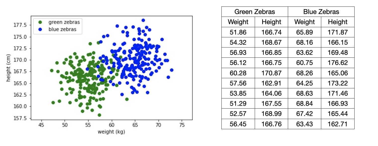
We want to know which of the features weight or height could be best used to characterize the difference between the two groups. To determine which of the two features is more informative we use, you guessed, the SNR, which measures the variance of the signal versus the variance of the noise. And the best part? it is that it is relatively easy to compute.
How do we compute SNR?
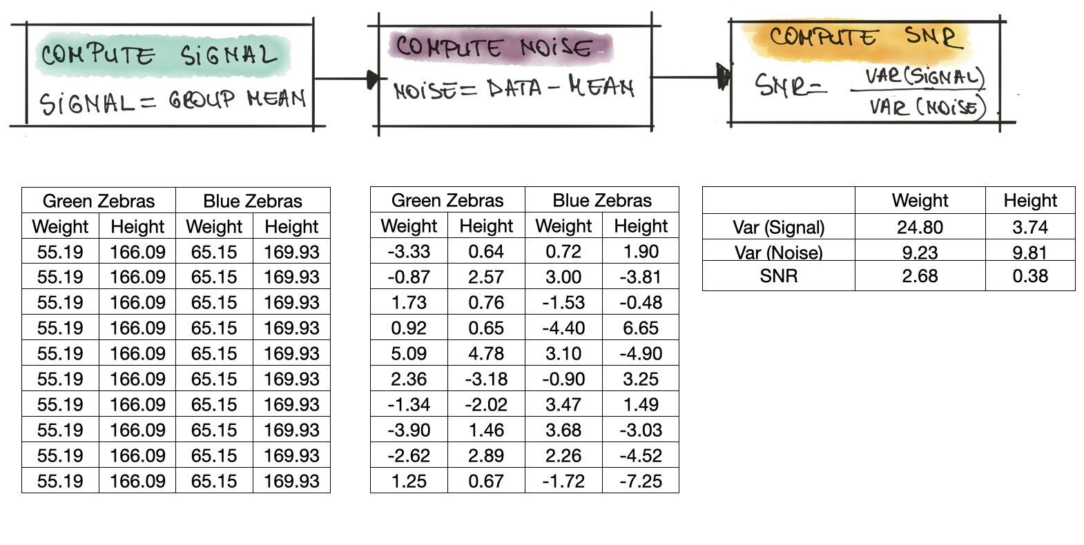
The SNR can be computed in three easy steps as shown in the figure below:
-
Compute signal for each group and each feature respectively. In our dataset of 400 zebras, the green zebras have an average weight of 55.19 kg and an average height of 166.09 cm. For the blue zebras, the average weight is 65.15 kg and the average height is 169.93 cm.
-
Compute noise i.e., how different are the measurements of one individual zebra from the average? To compute the noise, from each individual zebra we substract the mean.
-
To wrap things up, the formula used to compute SNR is listed below, where \(Var\) is the variance:
\[SNR=\frac{Var(Signal)}{Var(Noise)}\]
For our data, the SNR for the weight is 2.68 and is quite higher compared to the SNR for the height, which is 0.38. So, this SNR already tells us a bit about the data: very non-formally, it tells us that the weight of a zebra is more informative than their height (the SNR is a lot larger). Indeed, most zebras roughly the same height, but green zebras are lighter than blue zebras.
Our SCA data set
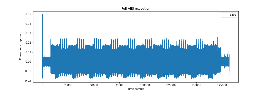
In the context of side channel analysis, our dataset is a set of power measurements and the features are the different time samples. For our example, we cloned the TinyAES implementation from this repository and loaded the firmware on an ARM Cortex M0, which was modified for the collection of traces. The set of traces we collected are available to you here. Below, an overview trace of the AES implementation, where you can clearly see the the individual AES rounds.
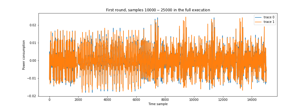
For this tutorial however, we focus on the first round, see below. We overlap two traces and check alignment. From what we see below we conclude that the traces are well behaved, meaning well aligned, so we can move on to the next step. As you know, DPA is a divide-and-conquer attack where we target one individual byte at a time. Lets assume our target byte is Byte 0 of the S-box out operation, Round 1 (in the notebook you can choose other values for the target byte). In the rest of the tutorial, we will refer to the target byte as $k$.
Computing SNR for the our SCA dataset
The only one difference to our first example when computing the SNR is that we now have to chose how to divide the traces in our data set in groups. Lets take a step and consider, what is the signal and what is the noise?
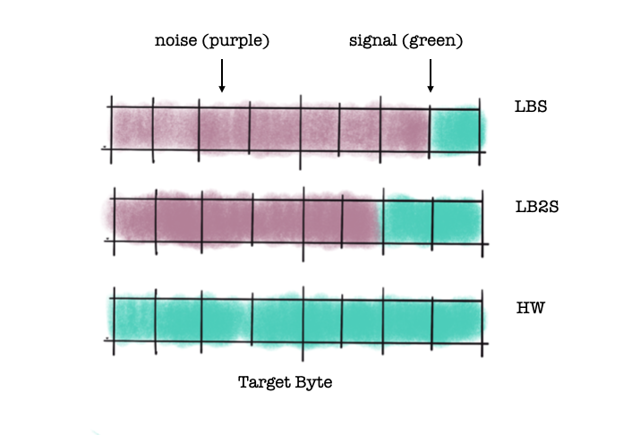
For side channels, very simply, the signal is the information exploitable for an attack and everything else is noise. Depending on the chosen leakage model, the same point (or time sample) may have different ratios of signal and noise as different attacks exploit different properties of the underlying operation. Of course, the more signal is present, the more easy an attack will be. In this tutorial, we compute and compare the SNR for three leakage models:
a) Least Significant Bit (LSB), which looks only at 1 bit of our target byte;
b) Least Significant 2 Bits (LS2B), which looks at the last 2 bits in the target byte;
c) Hamming Weight (HW), which looks at the number of ones in the target byte.
The figure below illustrates the exploitable information for our three chosen leakage models and we see that what we consider signal (green) or noise (purple) is determined by the choice of leakage model. SNR is computed independently for each time sample in the trace.
 The only missing ingredient now is how to prepare the data, which means to split the trace set according to the values associated with our leakage model. For example:
-
for the LSB leakage model, we create two groups, where $\text{LSB}(k)=0$ and $\text{LSB}(k)=1$
-
For the LS2B leakage model, we create four groups, where $\text{LSB}(k)=0$, $\text{LSB}(k)=1$, $\text{LSB}(k)=2$ and $\text{LSB}(k)=3.$
-
For the HW leakage model, we would split the trace set in 9 groups, where $\text{HW}(k)=0$, $\text{HW}(k)=1$, ..$\text{HW}(k)=8$
And voila:
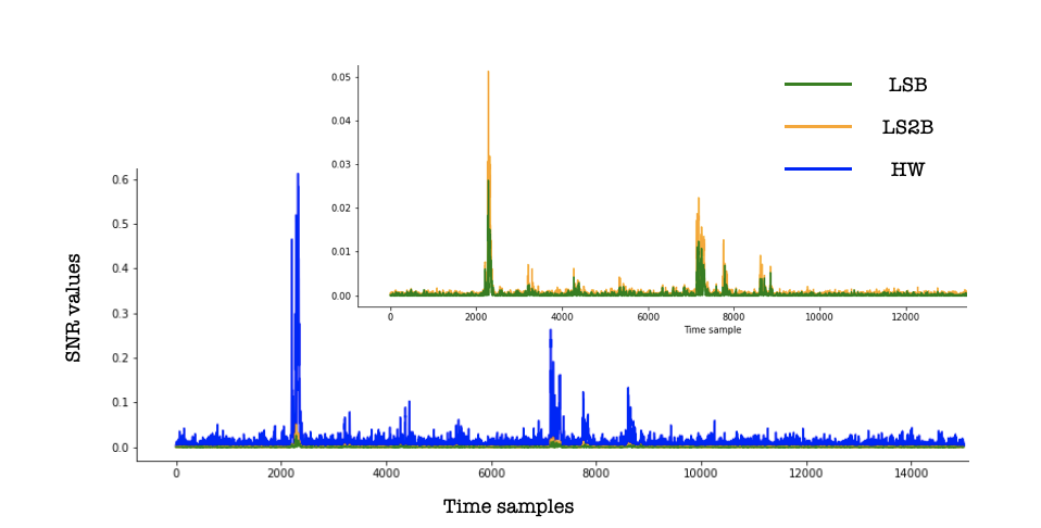
In this tutorial, we explored the use of SNR for choosing the best leakage model for a target. With our example, we can clearly see that the HW leakage model is more suitable than LSB or L2SB. It is worth highlighting that the SNR can have other applications such as estimating the quality of measurements, selecting points of interest (POI), or even key ranking/enumeration scenario as a pre-processing step (which we will explore in a future post).
Further reading materials:
- The concept of Signal-to-Noise Ratio (SNR) was first introduced to the area of side-channel analysis by Stefan Mangard in 2004 in his now classic paper Hardware Countermeasures against DPA - A statistical Analysis of Their Effectiveness. Definitely worth reading.
- An in-depth treatment of the subject can be found in Power Analysis Attacks, Revealing the Secrets of Smart Cards (Chapter 4), Stefan Mangard, Elisabeth Oswald and Thomas Popp.